Learn
Survey in, graded field out.
What RosettaGrade does, in the order you would do it — the workflow, the design types, how the volumes are computed, the water and the haul, the team, and exactly which files it will and will not write.
The workflow
Six steps, start to finish.
The office loop a land-forming contractor already works in. Every step runs in the browser; nothing about the field is uploaded in order to design it.
- 01
Bring a survey in
Start from field shots — the collector’s synced project, a CSV/XYZ point file, or any format we read: .ag3 projects, .ags / .agd, display multiplane text, LandXML, DXF, shapefile, GeoJSON, KML and elevation CSVs. A GeoTIFF DEM/DSM or a LAS point cloud comes in from inside an open project — Field ▸ Import surface — thinned to survey points. A point coded MB becomes the master benchmark; the rest build the surface. Units a file declares are read from the file; units it leaves ambiguous are yours to state.
- 02
Build the surface
The shots are triangulated into a constrained Delaunay TIN, clipped to the field perimeter, with breaklines held as constraints — so a levee or a ditch is enforced rather than smoothed away. Natural contours draw off the same surface the volumes are computed from; S-Contours smooths them at whatever interval you set, whole, single or partial, with nodes you can edit. A field with a georeferenced benchmark sits on aerial, road or hybrid imagery.
- 03
Split the field, if it needs it
Section lines and hinge lines divide a field into sections, each with its own design. A hinge lets two planes meet along a line you choose instead of at a fold the solver invented; hinged groups are solved together so every hinge stays continuous.
- 04
Design the grade
Pick the method for the job — see the design types below — and set the cut/fill ratio. The balancing elevation is solved for you, so the design lands on the ratio you asked for rather than on whatever the plane happened to give. Balance zones rebalance a ring on its own; drain-to-point, drain-to-linear and drain-to-edge reshape designed elevations toward a surveyed target; the target-ratio slider re-solves live; Variants compares several designs side by side.
- 05
Check the water and the haul
The water analysis fills the depressions, traces the flow paths and estimates a design storm’s runoff per pond, on the natural surface and again on the design. The haul estimate pairs cut with fill, draws the mass-haul diagram and the largest movements, and prices the job from your rates.
- 06
Check the yardage, then export
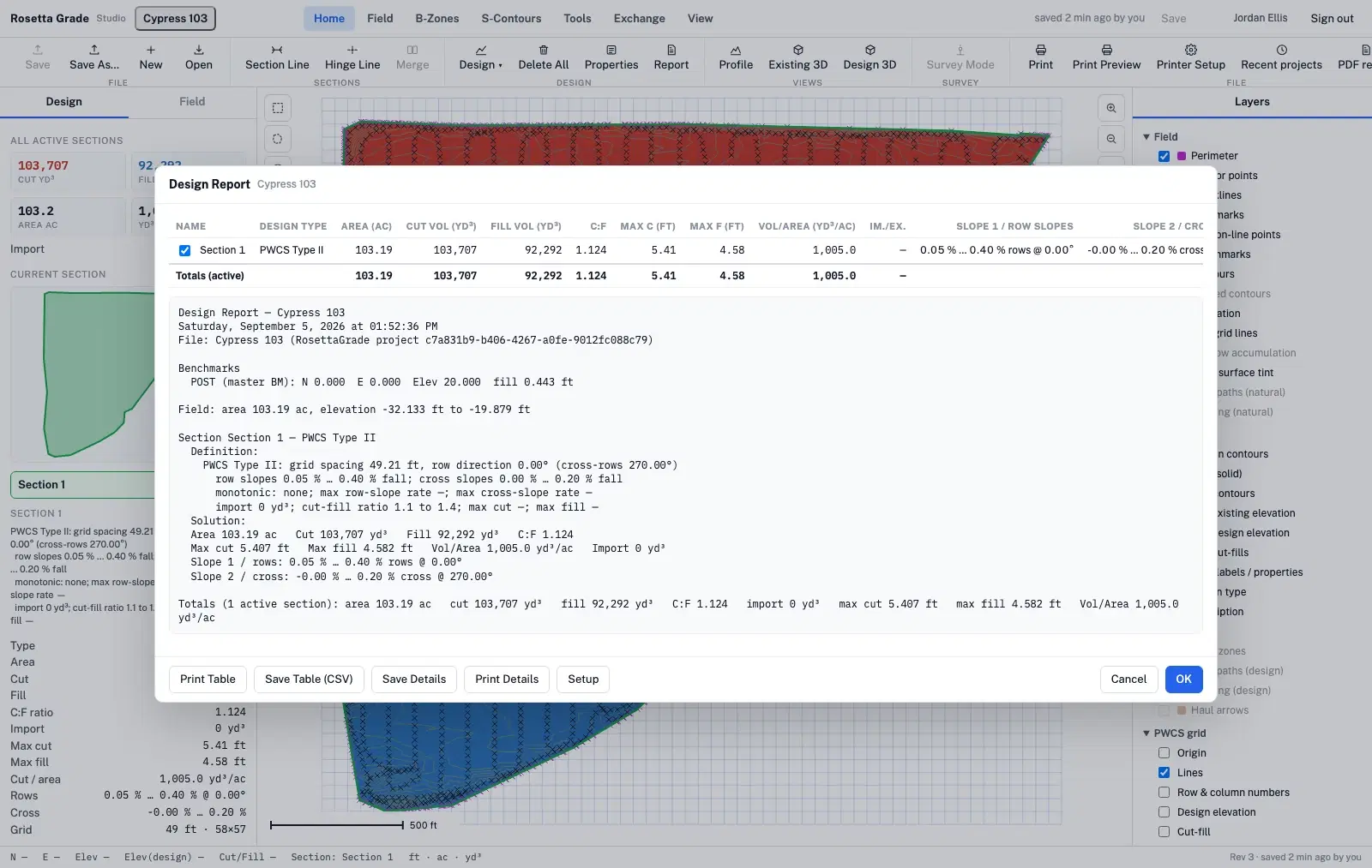
Cut and fill are computed as exact TIN prisms and reported with the ratio, the import/export term and the residual of the balance identity, so you can see the books close. Then write the design out: PWCS design and cut/fill grids, LandXML and DXF design surfaces, shapefile, KML, GeoJSON, design CSV, display multiplane text and point lists — or share a read-only link and a branded PDF of the report.
Design types
Pick the plane the field asks for.
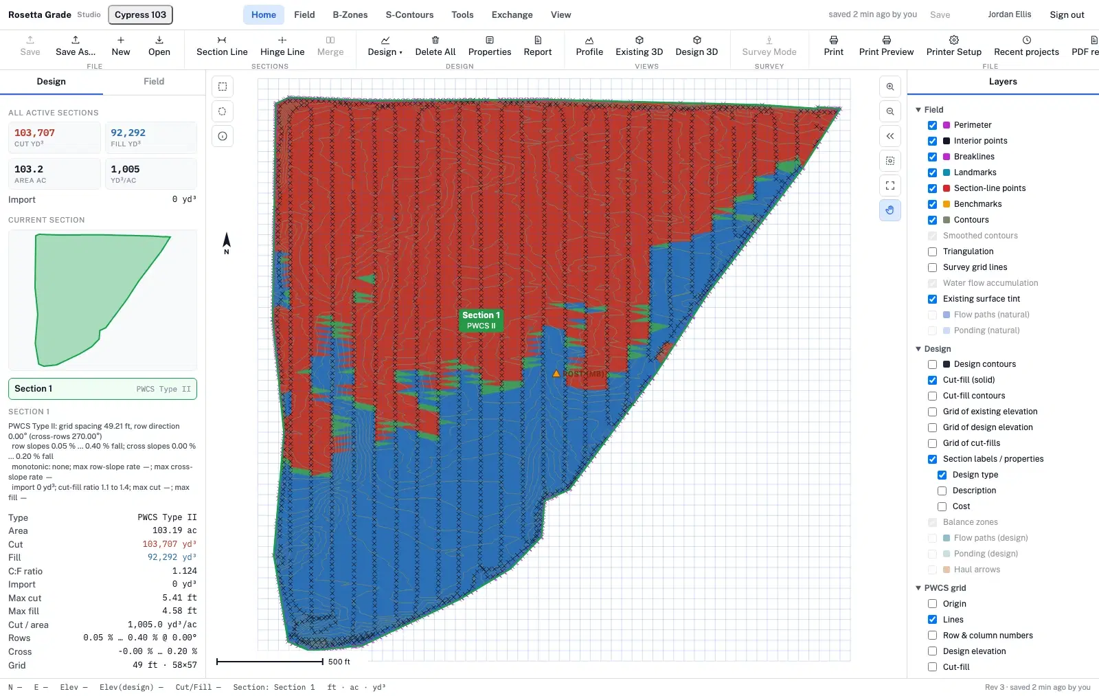
Each section of a field can carry its own design, so one job can mix a best-fit plane, a pinned tie-in and a variable-slope solve.
- Best-fit plane
- The least-squares plane through the surveyed surface, then shifted to your cut/fill ratio. The default starting point for most fields.
- Fixed slopes
- You set the row and cross-row slopes; the solver finds the elevation that balances at your ratio.
- Fixed point & slopes
- Both slopes and one pinned elevation — for a field that has to meet an existing structure, turnout or road.
- Hinged planes
- Two or more planes meeting along a hinge line you draw, best-fit or fixed-slope on each side, solved together across the whole hinged group.
- Matched to existing
- The design surface follows the existing ground, for edges and tie-ins that must not move.
- PWCS variable slope
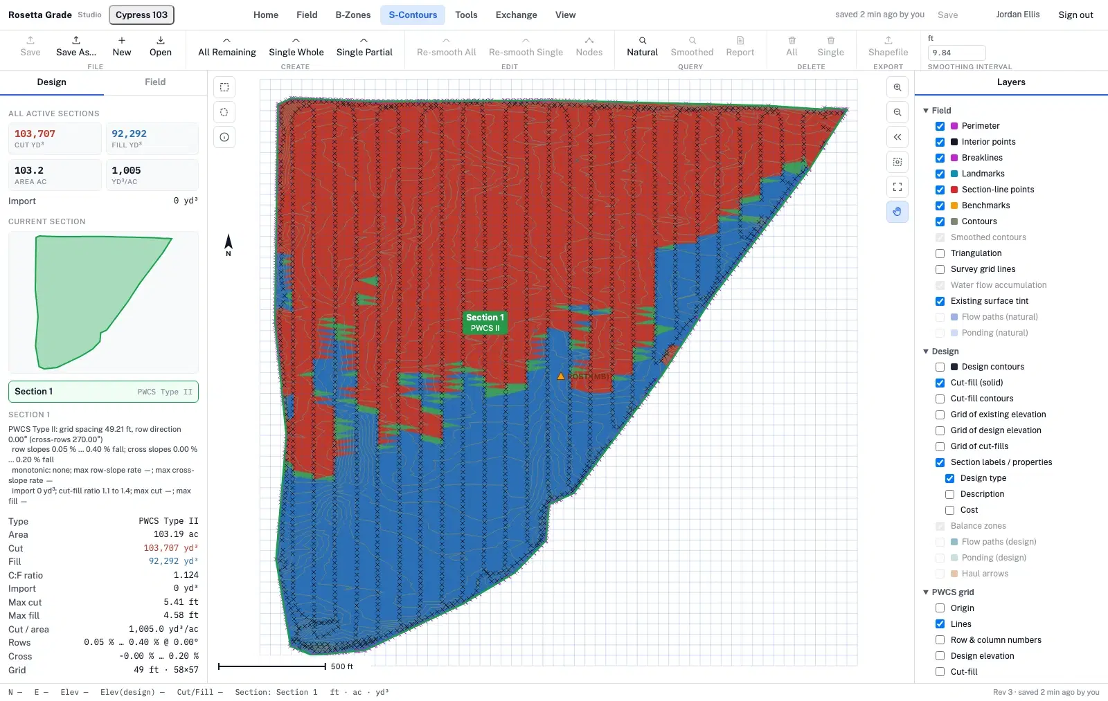
- Plane-with-continuously-varying-slope land grading, solved as a linear/mixed-integer program on a row × cross-row grid, in all eight variants, with slope bounds, monotonic rows, node constraints and max cut/fill. Every row is made to drain while the least soil moves. A 168-acre field solves in 2 s.
- Target ratio
- Not a type but a re-solve: drag the cut/fill ratio and the current design updates live with its volumes, max cut and haul, shrink and swell included, then applies as an undoable step.
Volumes
Cut and fill you can check line by line.
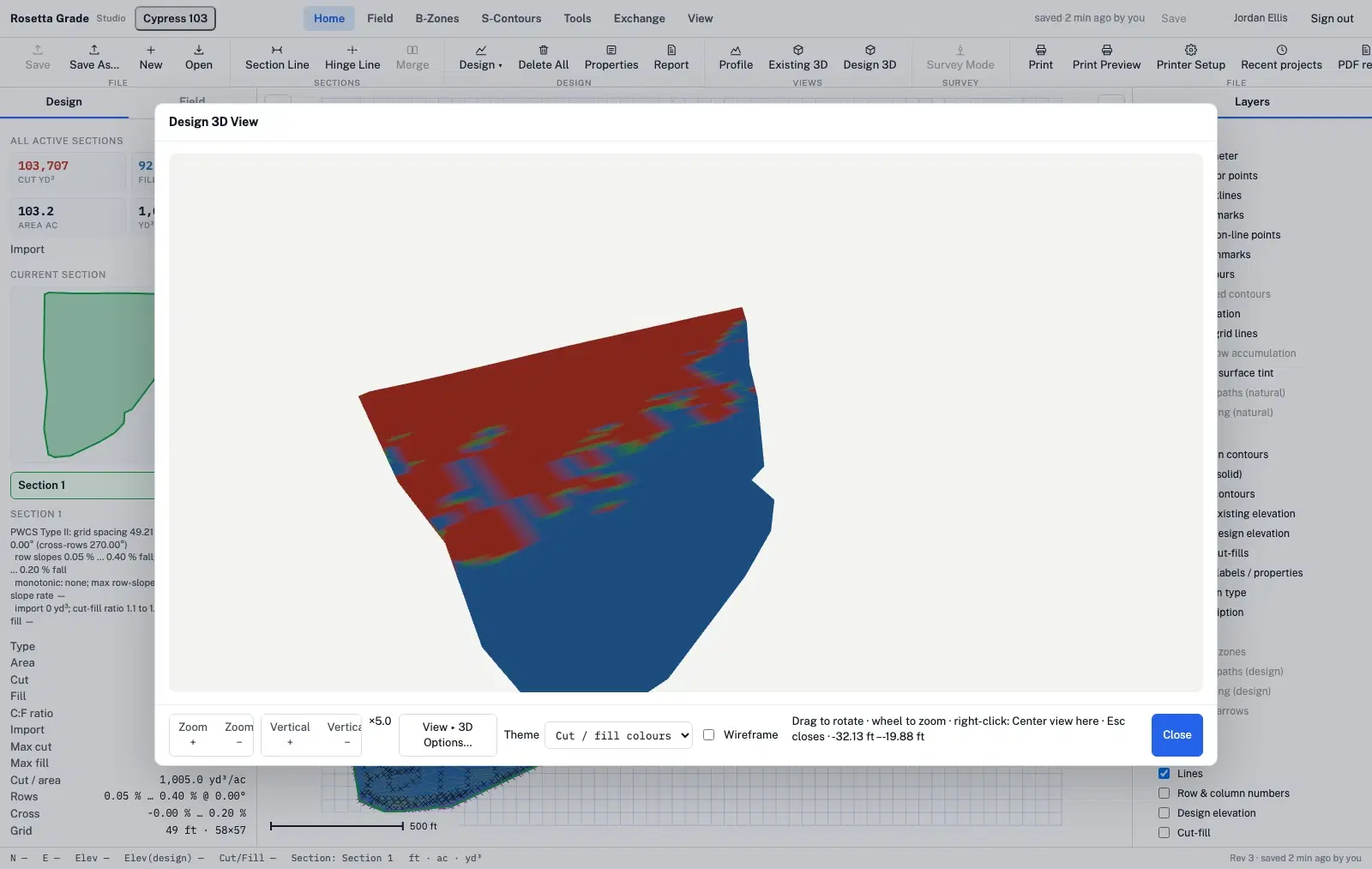
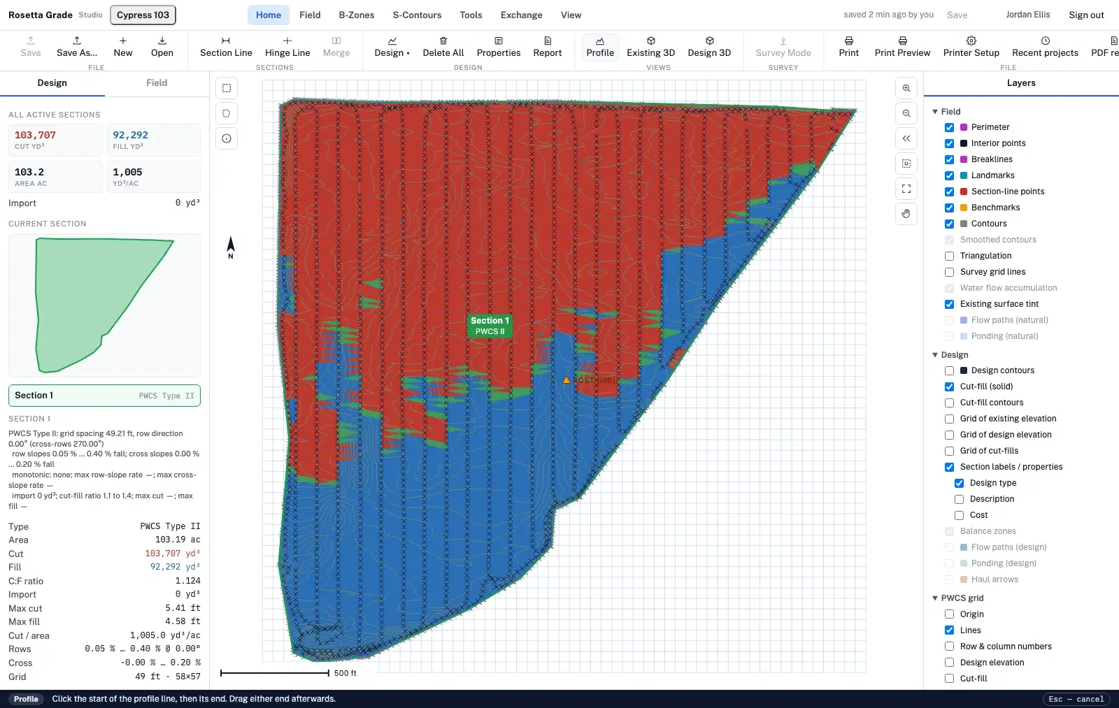
Volumes are computed as exact prisms between the existing TIN and the design surface — not sampled onto a grid and rounded until the two sides agree. Cut is red, fill is blue, and daylight — where the design meets the ground — is the line between them.
The design report prints the cut-fill balance identity, Vc − r·Vf + Vi = 0, together with its residual: cut volume, the cut/fill ratio you set, fill volume, and any import or export. If the residual is not effectively zero, the report says so rather than hiding it.
What else the report carries
- Area, cut and fill volume, cut/fill ratio, and cut per unit area.
- Maximum cut and maximum fill, so you can see the deepest move on the field.
- Row and cross-row slope ranges for the design, and the grid the solve ran on.
- The haul estimate and priced total, once you have computed them.
- Per-section and per-balance-zone figures when a field is split.
Water & haul
Where the water goes, and what the dirt costs to move.
Two analyses that run on the same surface as the volumes. Neither is saved as a guess: the water report lists every pond, and the haul is a pairing you can audit.
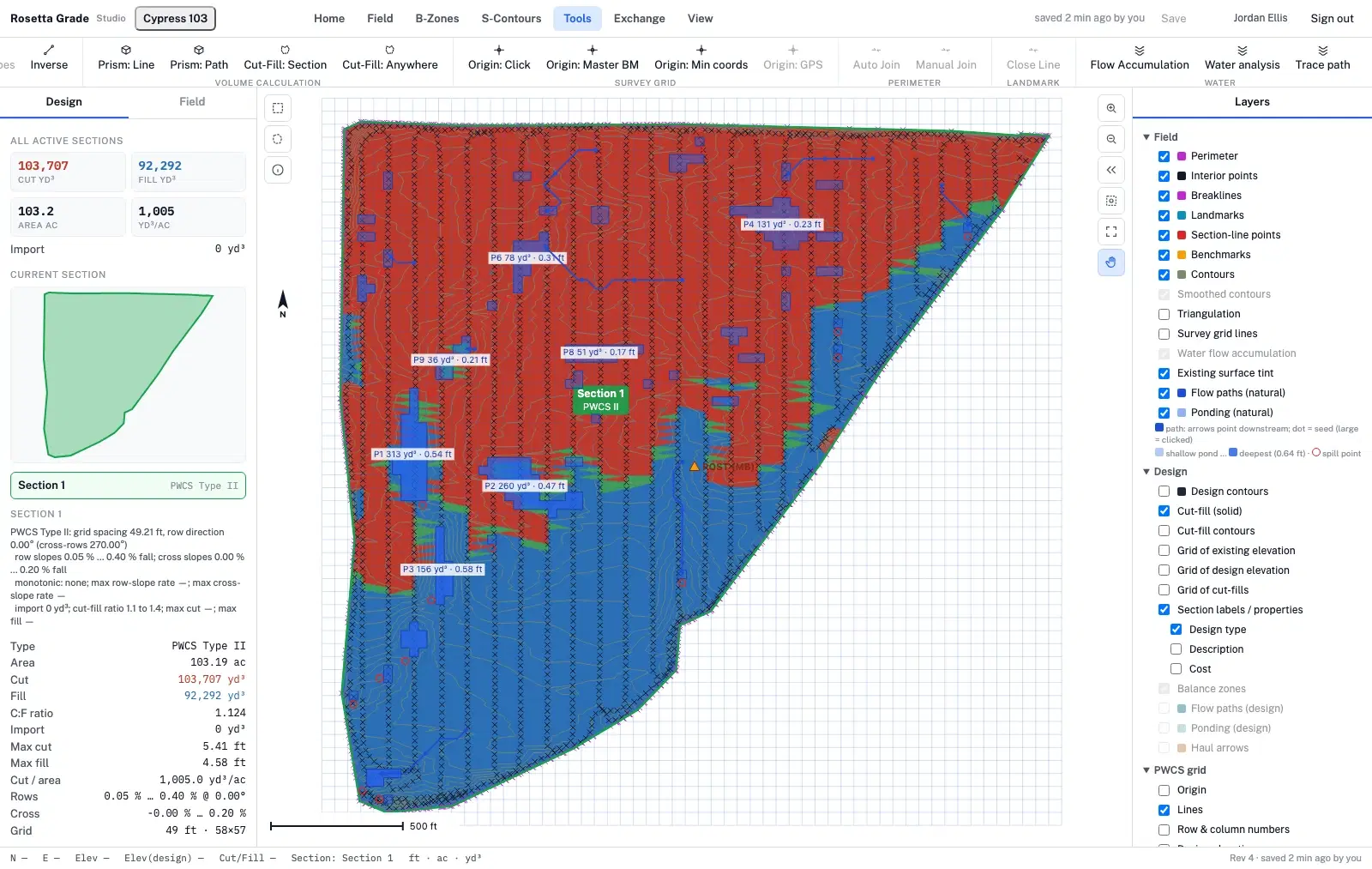
Water. Depressions are filled by priority-flood (Barnes 2014) into ponds with volume, maximum depth and spill point; flow paths are D8 lines seeded at the highest-accumulation cells or wherever you click; storm runoff uses the SCS curve number method (USDA TR-55) with a rainfall depth, duration and CN you set. Run it on the natural surface and on the design to prove the ponds are gone.
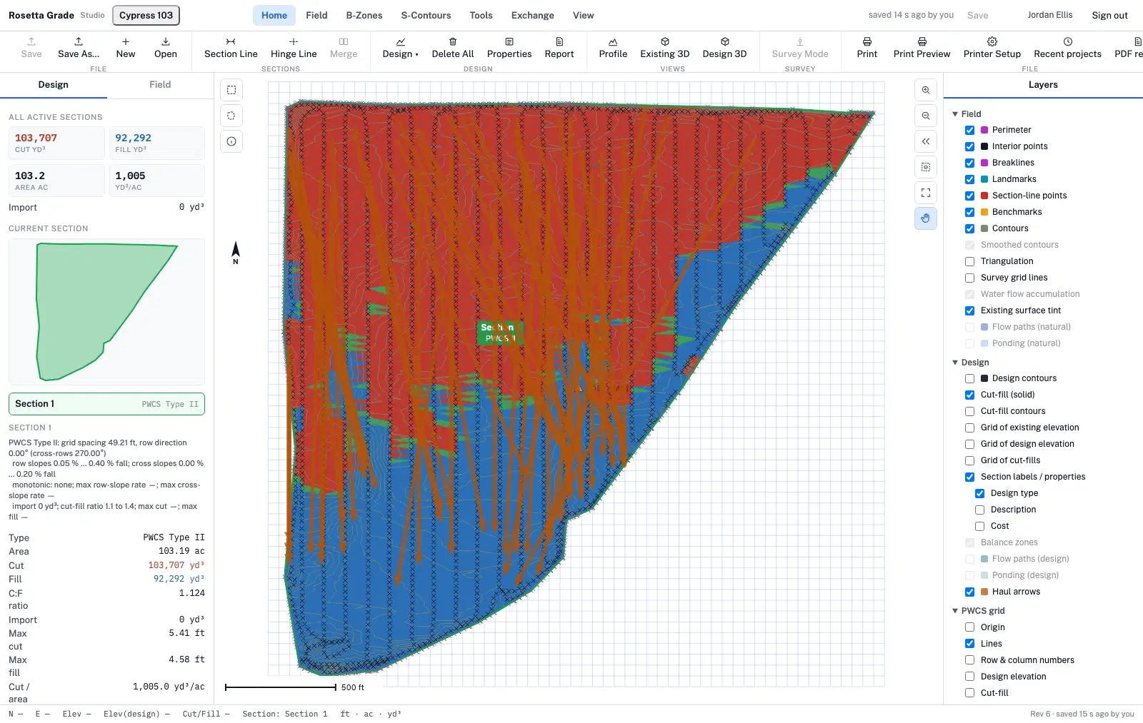
Haul. Cut cells are paired with the nearest fill cells (cut needed = ratio × fill) and the pairing is improved by 2-opt exchange — an approximation of the transportation optimum, not a machine plan. The result is haul in yd³·ft and yd³·mi, the average and longest haul, a mass-haul diagram along the rows and a priced estimate from your cost per yd³ of cut, per yd³·mi of haul and mobilisation.
Teams & sharing
The library is the office.
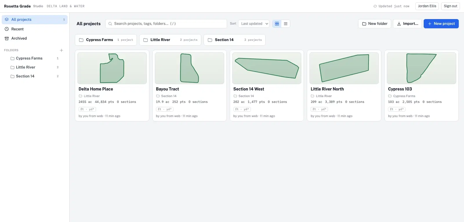
Projects save to your company’s library with folders, thumbnails, area and point counts. Every save is a revision you can restore; project locks show who is editing; other browsers see a save the moment it lands.
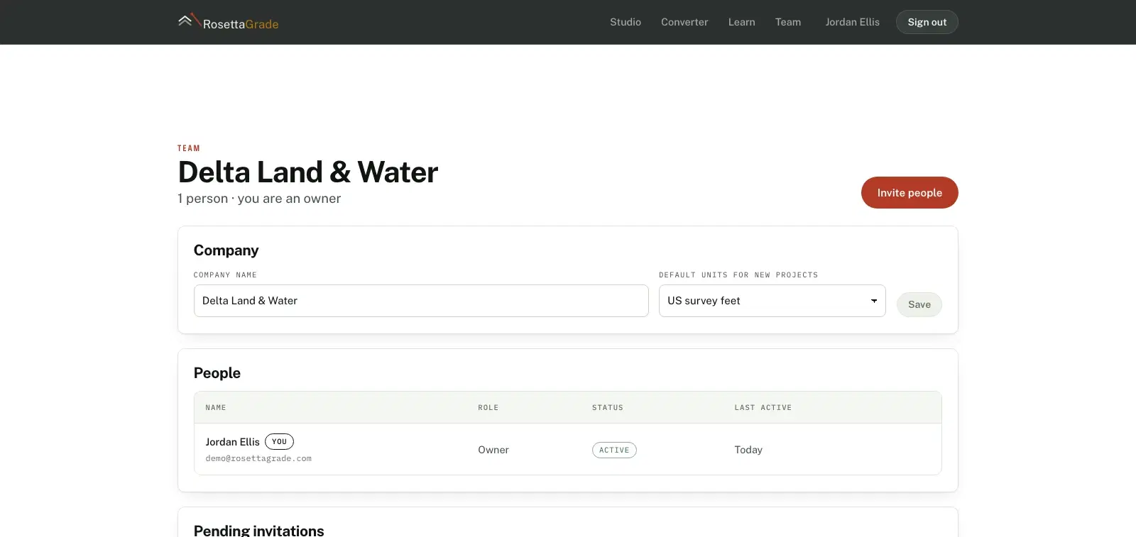
- Roles. Owner and admin run the company; designers create and edit projects and export files; surveyors collect and upload surveys and edit the projects they work on; viewers open projects and reports and cannot change anything.
- Share. A share link gives a public read-only view of the report and a map snapshot, revocable from the same place, and the PDF report is built in the browser.
- Audit. The activity feed on every project and the company audit log record who did what, when and from where.
In development · preview build
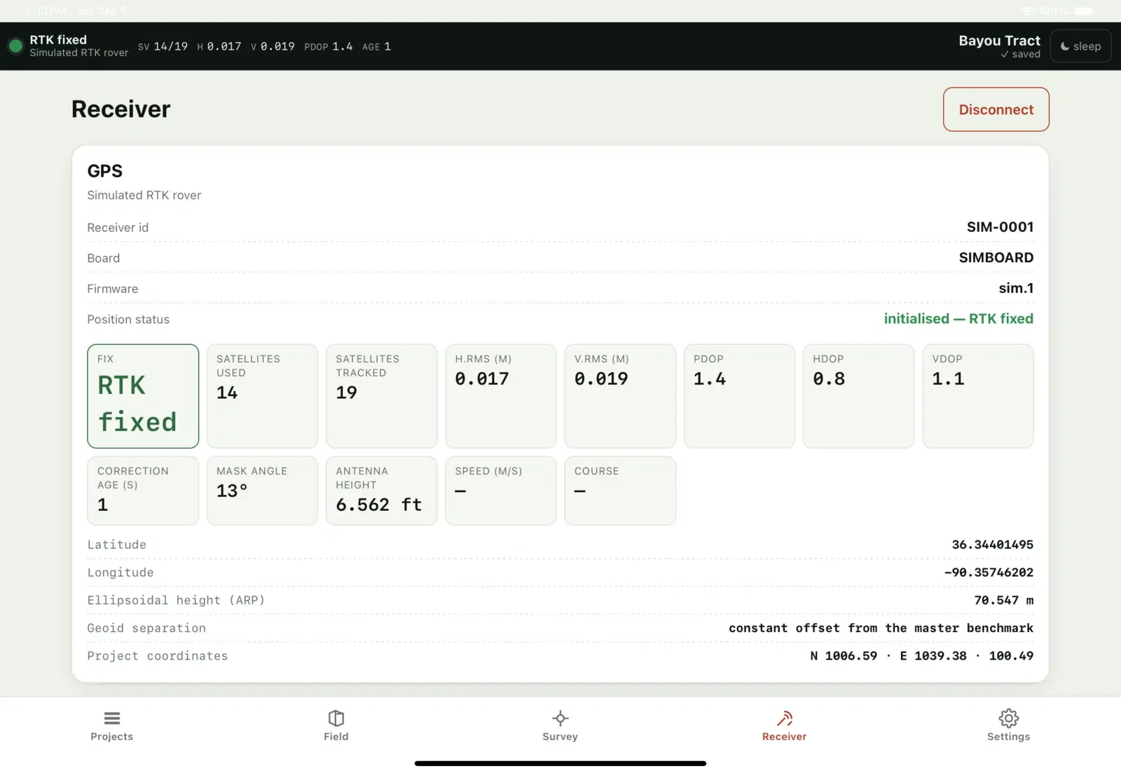
The collector, in brief.
An iPad and iPhone survey app that connects to an RTK rover, records benchmarks, perimeter, interior, breaklines and landmarks with a quality gate on every shot, and syncs the project to the Studio library. The preview shown here runs on its built-in RTK simulator; it has not yet been bench-tested with a physical receiver, and there is nothing to download today.
The converter
Every conversion is labelled before you download it.
The converter inspects the file first — format, point count, units, benchmark, surfaces, boundaries — then tells you what each possible destination would keep and what it would lose. The label is a promise, not a mood.
Two rules sit underneath those labels. A void stays a void: where a surface has no data, we write no data — never 0.00, the substitution that turns a design into a hole in a field. And we never write a machine-control format we cannot verify: an undocumented binary that a tractor would run on is read for inspection and refused for output.
Formats
Thirteen formats read, eleven written.
Generated from the converter’s own registry, sorted by how much we can prove. Open specifications first, then formats verified against real files, then formats whose structure is not fully documented — and last, the ones we read but will not write.
| Format | Extensions | Support | What we can prove |
|---|---|---|---|
| AutoCAD DXF (ASCII) | .dxf | Read + write | Open specification — implemented completely. The surveyor and CAD bridge. Reads POINT, LINE, POLYLINE and 3DFACE (welded into a TIN); writes R12-compatible ASCII with codes as layer names. No georeference — coordinates pass through as drawn. |
| ESRI Shapefile (.shp + .shx + .dbf) | .shp .dbf | Read + write | Open specification — implemented completely. The bridge to GIS and farm-management software — the mapping tools and the major farm platforms all speak it. Reads points, lines and polygons with .dbf attributes; writes a WGS84 PointZ set with .shx/.dbf/.prj. Upload the .shp, .shx and .dbf together. |
| Generic survey points (x, y, z, description) | .xyz .csv .txt | Read + write | Open specification — implemented completely. The lowest common denominator. Almost every RTK receiver and design package reads it. No benchmark semantics, no units declaration — carry those out of band. |
| GeoJSON (RFC 7946) | .geojson .json | Read + write | Open specification — implemented completely. The way out of the land-forming silo and into FMIS, GIS and web mapping. WGS84 only — a job with no geographic reference cannot be exported here. |
| Google Earth KML | .kml | Read + write | Open specification — implemented completely. The share-with-anyone format: opens in Google Earth and most GIS. WGS84 lon/lat/alt, points and linework only — no TIN, and a job with no geographic reference cannot be written. |
| LandXML 1.2 | .xml .landxml | Read + write | Open specification — implemented completely. The open hub format. Carries a real TIN, breaklines, boundaries and declared units. Has no native master-benchmark concept — we preserve it as a coded point. |
| Survey file (.ags) | .ags | Read + write | Verified against real files. Column order Lat, Long, Elev, Code, per the published import list for this format. Geographic, so it georeferences cleanly, but has no explicit master-benchmark record. |
| Land-forming point list (Pt, E, N, Elev, Ident) | .txt .csv | Read + write | Verified against real files. A plain-text point list in the column order these design packages expect, for moving a finished design between them. |
| Display survey, multiplane text (multiplane.txt) | .txt | Read + write | Verified against real files. Local coordinates relative to the master benchmark, true-north oriented. Layout published by Foresoft in the EziGrade importer documentation. |
| Design file (.agd) | .agd | Read + write | Not fully documented — check the notes on every conversion. The design-surface version of the AGPS file. Written by the same reader the survey file was verified with; double-check the first one on a test pass before it goes to a machine. |
| Farm-software elevation export (.csv) | .csv | Read + write | Not fully documented — check the notes on every conversion. Header-driven. These export column names vary by product and release, so columns are matched by name rather than position. Verify the elevation column on first use for a given export. |
| Land-forming project (.ag3) | .ag3 | Read only | Not fully documented — check the notes on every conversion. Tagged block store, decoded from real files and validated across versions 1.18, 2.1, 2.3, 4.1 and 5.0 — one container, one code path. Vertices (metres), the TIN including neighbour topology, benchmarks (local coordinates, latitude/longitude in radians, description, and the file's own master-benchmark flag), the shot table with each shot's layer (perimeter / breaklines / landmarks / section lines) and timestamp, and the layer table are recovered. So is the DESIGN: the graded design is never a second triangulation — it is held per section as an outline, a height at the local origin and two slopes — and those are read and checked against the surveyor's own printed sheets. So are the VARIABLE-SLOPE (PWCS) sections, which the section table does not hold at all: their outline, slope band and solved node grid come out of the file's tag 23/24/25 blocks, together with the design's own area, volumes and maximum cut/fill. Matched designs are not decoded; sections holding one arrive named and outlined but ungraded, and say so. Read only — no writer, because a control file we cannot verify against vendor software is a field-scale risk. |
| Machine-control design file (.gps) | .gps | Read only | Undocumented binary — inspection only. Undocumented binary holding a gridded design surface, a cut/fill grid and the natural surface, all relative to an embedded master benchmark. Read for inspection only — we will not write a file a tractor runs on that we cannot verify. |
The Studio additionally imports GeoTIFF DEM / DSM rasters and LAS point clouds, thinned to survey points, from Field ▸ Import surface inside an open project; those are one-way imports and are not part of the converter.
File extensions and format names are used only to say what RosettaGrade is compatible with. Any third-party product or format name that appears anywhere on this site is the trademark of its owner. RosettaGrade is an independent product of Real World Development and is not affiliated with, endorsed by or sponsored by any of them.