Variable-slope grading
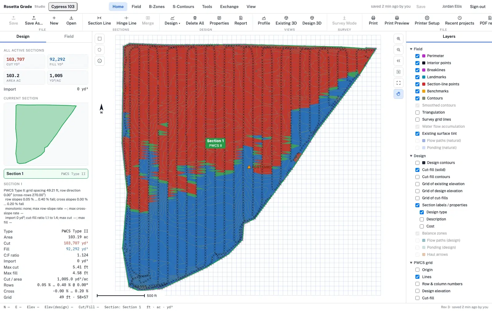
Plane-with-continuously-varying-slope grading in all eight variants, with slope bounds, monotonic rows, node constraints and max cut/fill, solved as an LP/MIP in your tab.
Survey → Design → Machine control
RosettaGrade Studio imports your field survey, builds the terrain model, solves the grading design, shows you the water and the haul, and writes files your display and your office can actually run — with nothing to install and nothing to licence per machine.
Terrain model, design solve, water analysis and volumes run in your tab. Nothing about your field is uploaded to design it.
Survey → Design → Machine control
The office loop a land-forming contractor already works in, with the field and the office on the same screen.
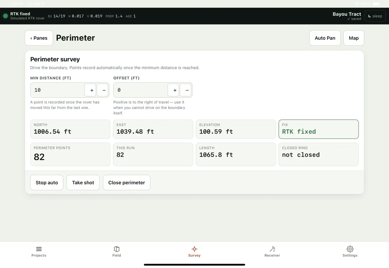
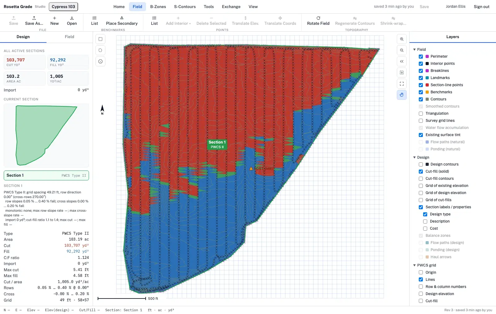
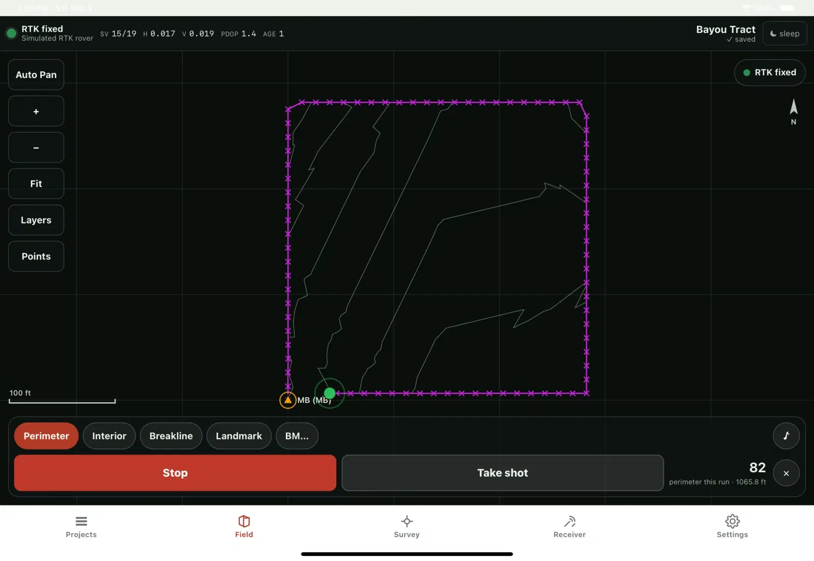
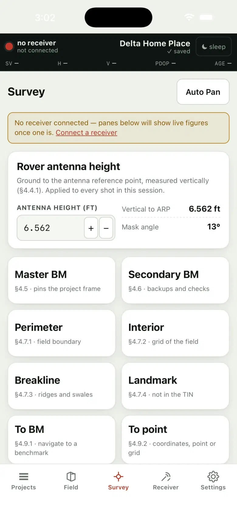
The iPad and iPhone collector records master and secondary benchmarks, perimeter, interior, breakline and landmark shots from an RTK rover — auto-shot by distance, every shot gated on fix quality. Or import what you already have: an .ag3 project, a display multiplane file, LandXML, DXF, shapefile, GeoJSON, KML or a CSV of points. A GeoTIFF DEM or a LAS point cloud comes in from inside a project — Field ▸ Import surface — where you choose how it is thinned to survey points.
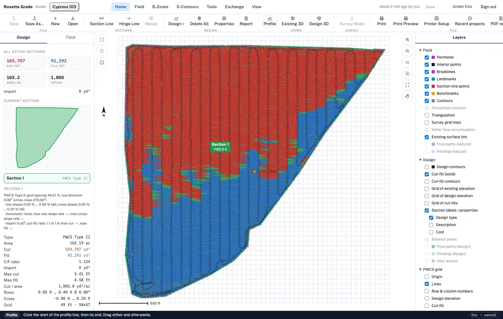
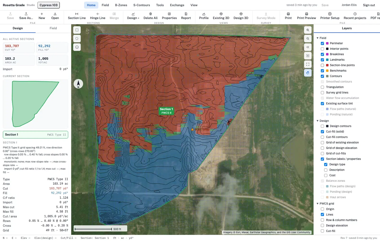
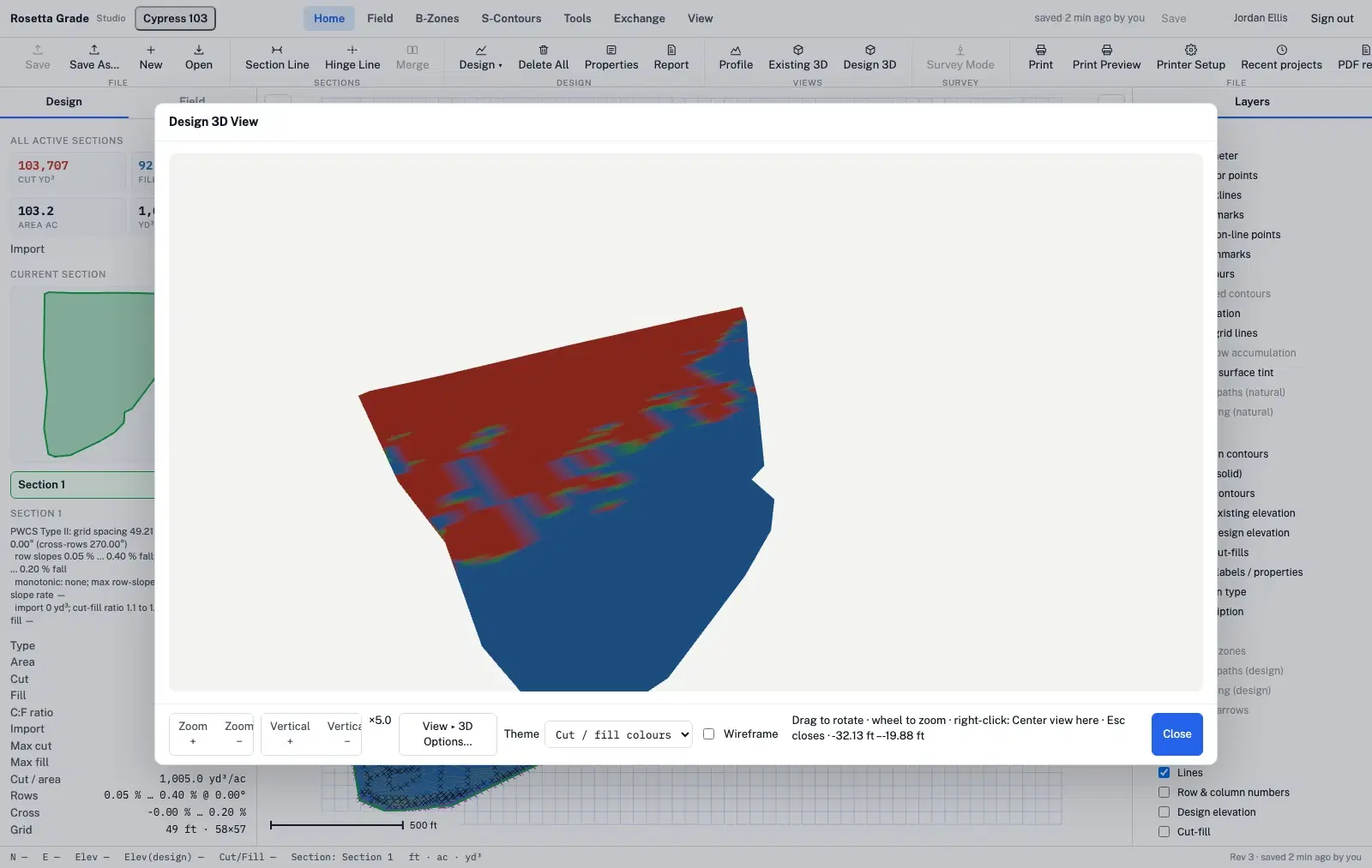
Best-fit, fixed-slope, fixed-point, hinged and matched planes across any number of sections, or a PWCS variable-slope design in all eight variants, solved as a linear program in the tab. Cut and fill are exact TIN prisms. Cut a profile through the design, orbit it in 3D, drag the target-ratio slider and watch the volumes re-solve.
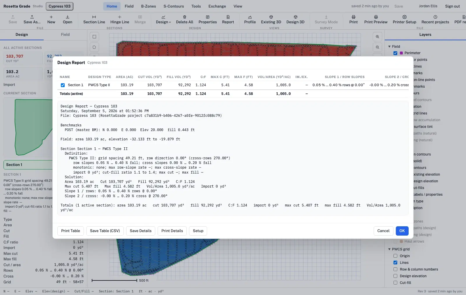
The design report prints every section with area, cut, fill, ratio, maximum cut and fill, slopes and the haul estimate, and it prints the residual of the cut-fill balance identity so you watch the books close. Then write the job out: design and cut/fill grids for the display, LandXML and DXF surfaces, shapefile, KML, GeoJSON, elevation CSV, multiplane text and point lists.
Water analysis
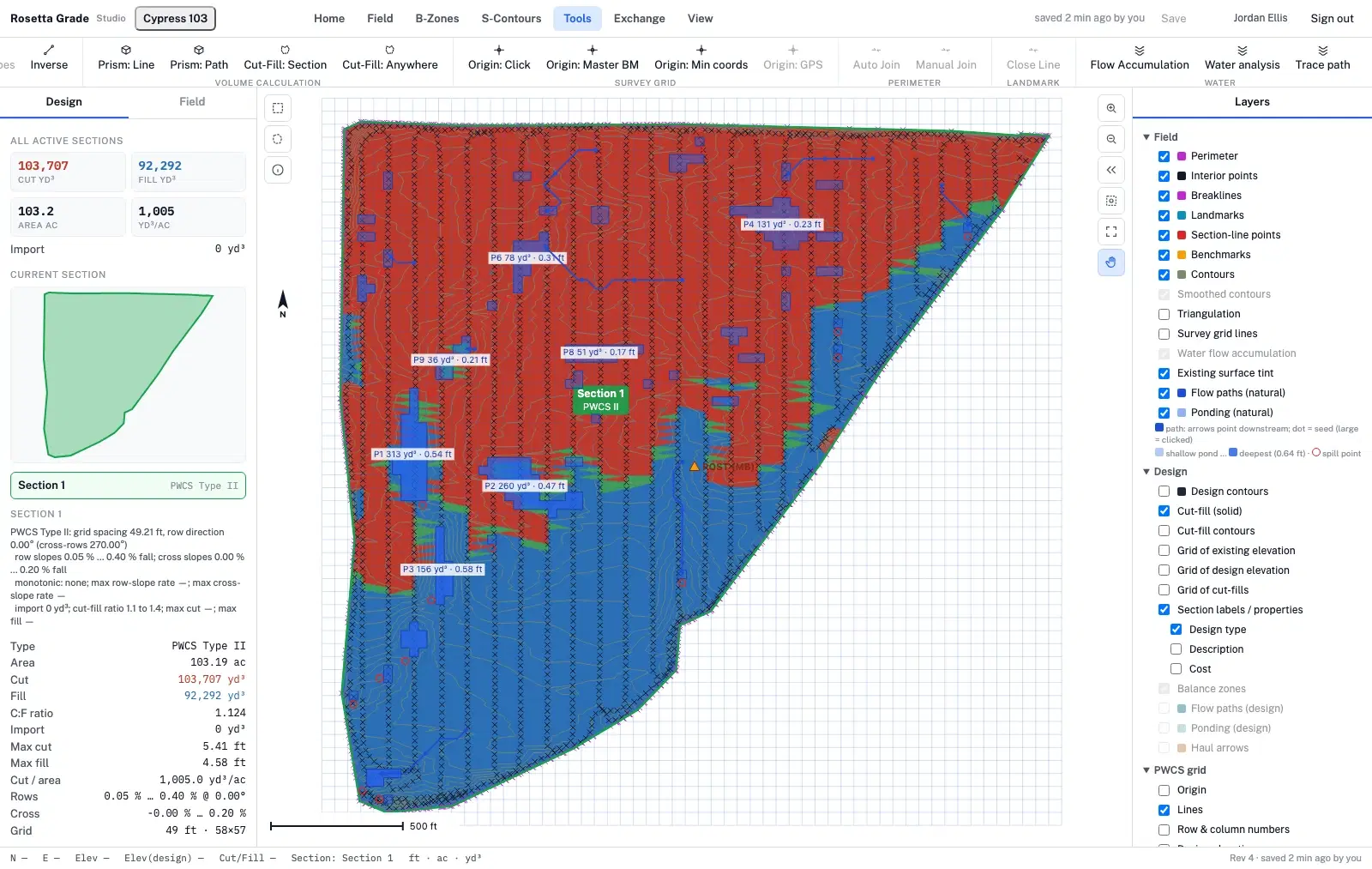
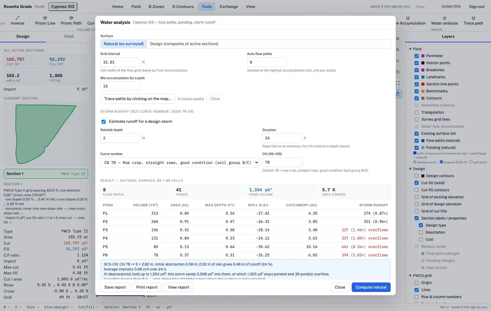
The water analysis fills every depression on the surface (priority-flood), traces the D8 flow paths to their outlets, and sizes a design storm’s runoff per pond catchment with the SCS curve-number method. Run it on the natural ground to see the problem, and on the design to prove it is gone.
Every pond is a row: volume, area, maximum depth, spill elevation, catchment and the storm runoff it receives — with the ponds that overflow called out. The verdict at the bottom says whether the drainage is adequate, in words.
Haul & cost
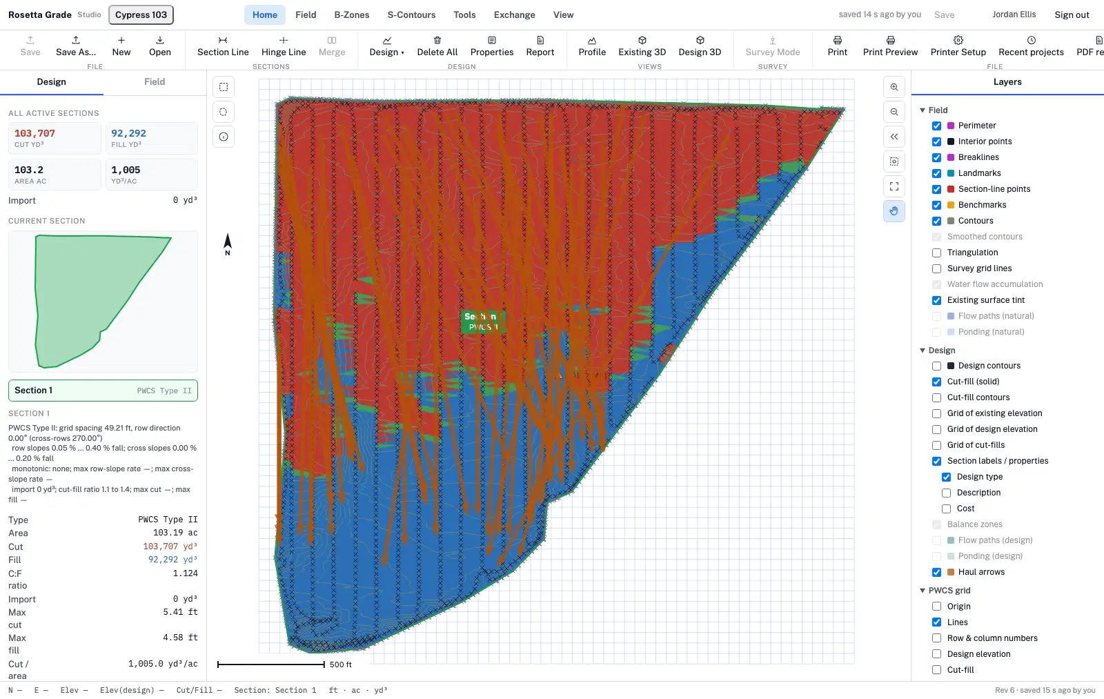
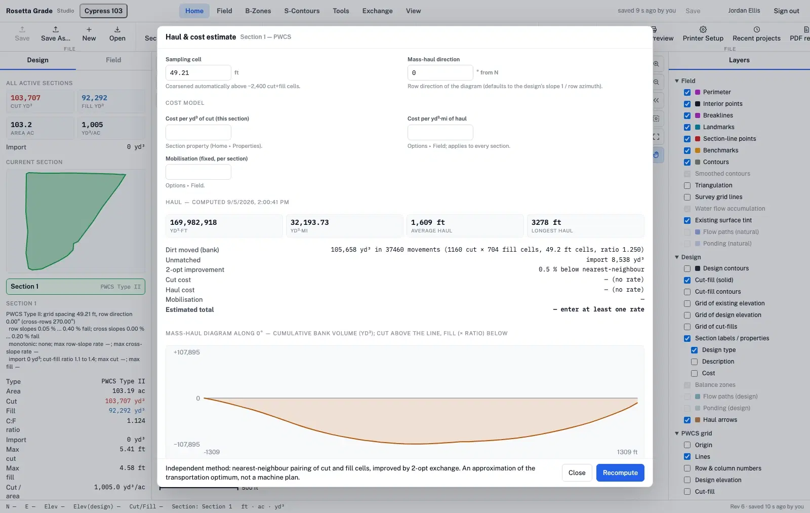
The haul estimate pairs every cut cell with the nearest fill (cut needed = ratio × fill), improves the pairing by 2-opt exchange, and reports the haul in yd³·ft and yd³·mi, the average and longest haul, a mass-haul diagram along the rows, and the fifty largest movements as arrows on the map. Enter your rates and it prices the job.
Cost per yd³ of cut, cost per yd³·mi of haul and a mobilisation charge — each one a project or section property you set once — give an estimated total next to the cumulative bank-volume curve.
The surface
Shots are triangulated into a constrained Delaunay TIN, clipped to the perimeter and pinned to the breaklines, so a levee or a ditch stays where you surveyed it. Contours, profiles, 3D and volumes all come off the same surface.
Everything the job needs
The design types, contours, balance zones and reports a land-former expects — plus water, haul, imagery, DEM import, teams and sharing on top.
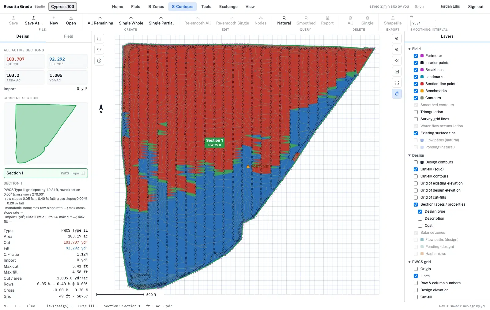
Plane-with-continuously-varying-slope grading in all eight variants, with slope bounds, monotonic rows, node constraints and max cut/fill, solved as an LP/MIP in your tab.
Best-fit or fixed-slope planes that meet along hinge lines you draw, solved together so every hinge stays continuous; matched designs for edges that must not move.
Draw a balance-zone ring and the solver rebalances inside it, so a haul-limited corner pays for itself instead of borrowing dirt from the far end of the field.
Drag the cut/fill ratio and the design re-solves live with the volumes, max cut and haul updating — shrink and swell included — then apply it as an undoable step.
Natural contours off the TIN, then S-Contours smoothed at the interval you choose — whole, single or partial — with nodes you can edit and a shapefile export for the levee crew.
Priority-flood depressions with volume, depth and spill point, D8 flow paths, and SCS curve-number storm runoff per pond catchment — on the natural surface and on the design.
Cut cells paired to the nearest fill and improved by 2-opt exchange: haul in yd³·ft and yd³·mi, average and longest haul, a mass-haul diagram along the rows, the 50 largest movements as arrows, and a priced estimate.
Aerial, road and hybrid basemaps under any field with a georeferenced master benchmark, with linework colours you can pick to stay legible over imagery.
A GeoTIFF DEM or DSM, or a LAS point cloud with ground classification, thinned to survey points and placed through the project’s master benchmark.
Owner, admin, designer, surveyor and viewer roles for the company, with invitations, folders, an activity feed and an audit log of who changed what.
Every save is a revision you can restore. Project locks show who is editing, and other browsers see the save the moment it lands.
A public read-only link to the report and a map snapshot — revocable — and a branded PDF of the design report built in the browser.
Teams
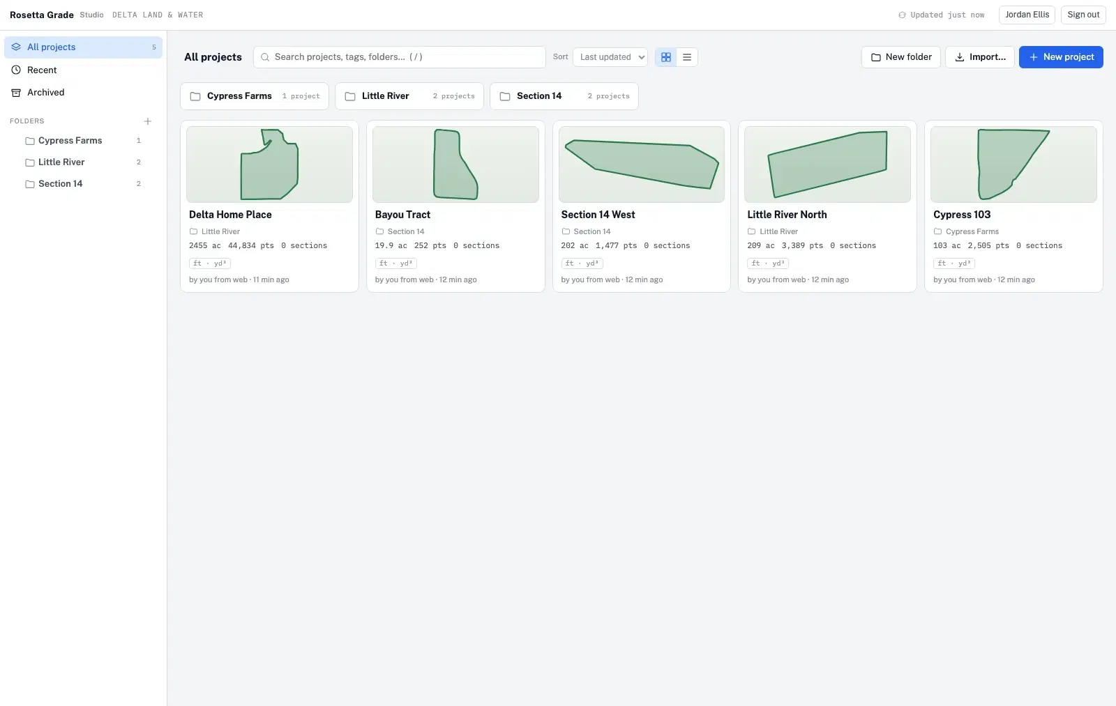
Projects live in folders with a thumbnail, the area, the point count and who saved them last. Every save is a revision; every change is in the audit log; a share link gives the customer the report without an account.
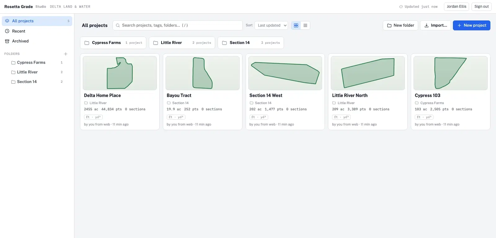
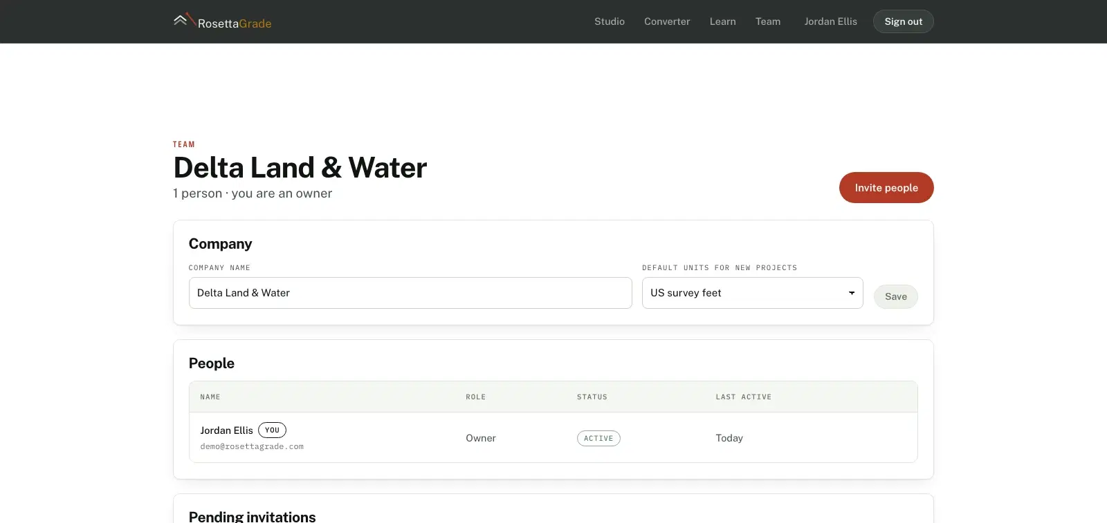
The admin dashboard shows the whole installation: users, invitations, organisations, projects and the storage they take, saves and sign-ins by day, live editing locks, mail failures, recent activity and health checks — so the person who runs the company can answer “what happened?” without asking us.
In development · preview build
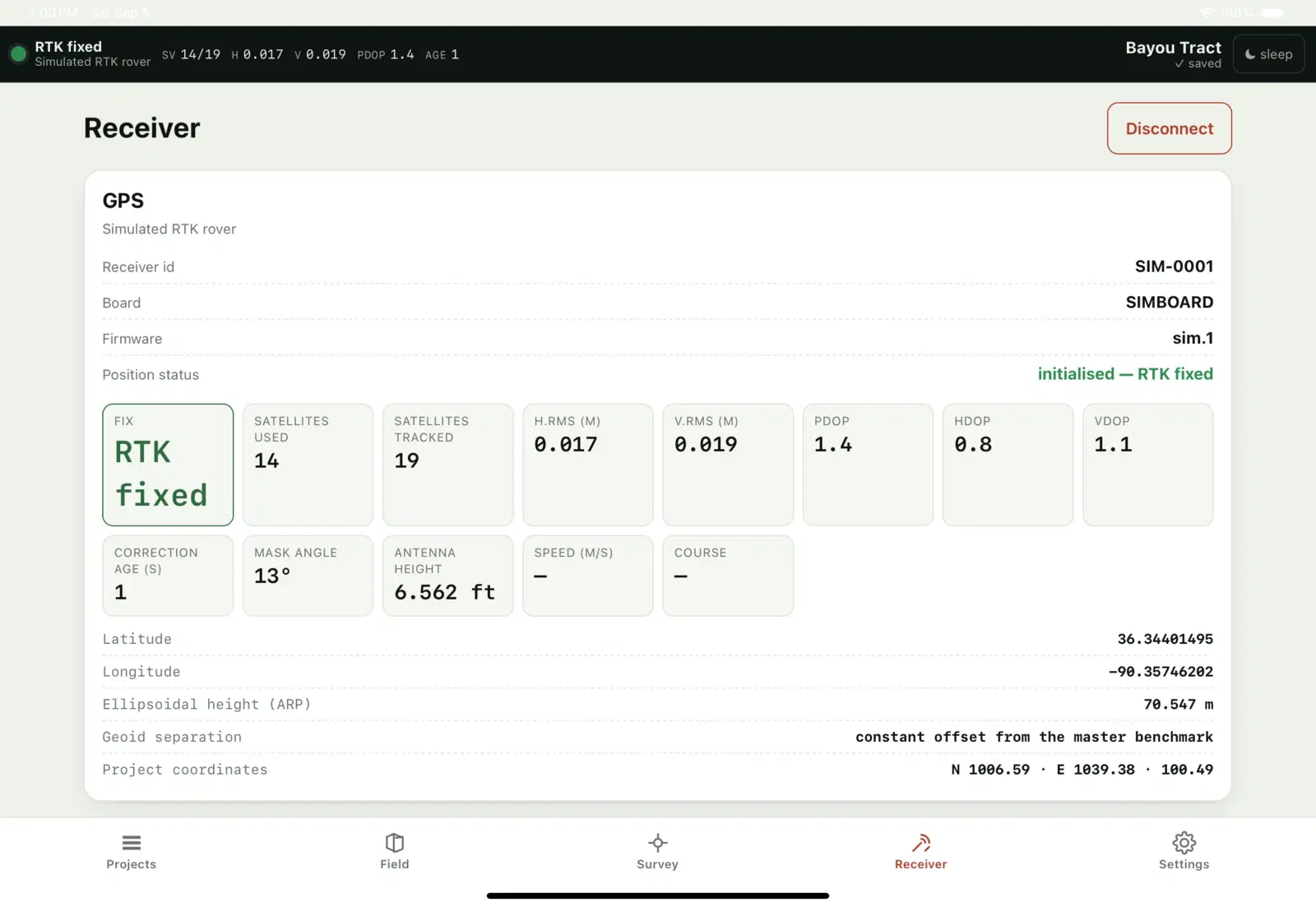
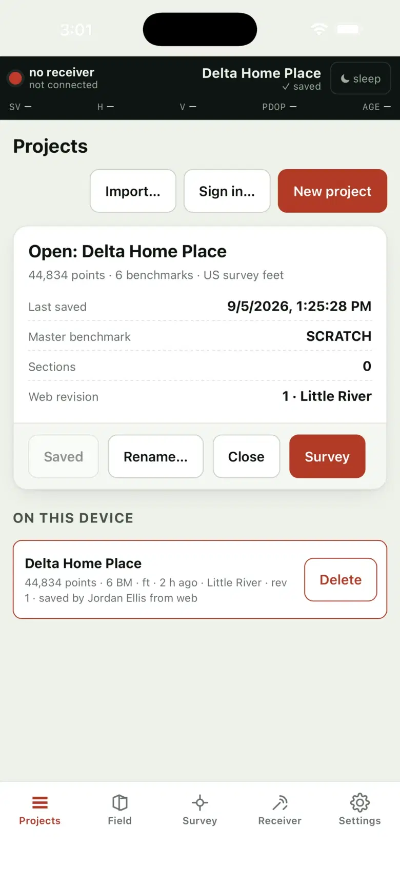
The other half of the loop: an RTK survey app for iPad and iPhone that shoots the field and syncs the project straight into the Studio library. What you see here is the working preview driven by its built-in RTK simulator — it has not yet been bench-tested against a physical receiver, and there is nothing to download today.
The converter
The file converter reads thirteen formats and writes eleven. Before you convert, it inspects the file, shows you what is in it, and stamps the conversion with an honest label — because the expensive mistake in this industry is a file that looked fine. Unlike the Studio, the converter does its reading and writing on our server: the file you drop is uploaded, converted and handed back.
What it is
Survey in, balanced design out, with the water and the haul on the way — and the files your display reads at the end of it. Here is the whole of it, including the one thing it does not do.
| Runs on | Any current browser — macOS, Windows, Linux, ChromeOS, iPad. No install, no licence file, no per-machine version to keep in step. |
|---|---|
| Variable-grade design | Plane-with-continuously-varying-slope in all eight variants, solved as a linear program in the tab, with slope bounds, monotonic rows and max cut/fill. |
| Planes and hinges | Best-fit, fixed-slope, fixed-point, hinged and matched planes across any number of sections, solved together so every hinge stays continuous. |
| Volumes | Exact TIN prisms against the surveyed surface, with the balance-identity residual printed in every report. |
| Haul | Cut paired to fill and improved by 2-opt exchange: yd³·ft and yd³·mi, average and longest haul, a mass-haul diagram, and a priced estimate from your rates. |
| Water | Priority-flood ponding with volume, depth and spill point, D8 flow paths, and SCS curve-number storm runoff per catchment — on the natural ground and on the design. |
| Imagery and elevation data | Aerial, road and hybrid basemaps under any georeferenced field; GeoTIFF DEM/DSM and LAS point clouds thinned to survey points. |
| Working together | One library for the company: folders, revisions on every save, editing locks, roles, an audit log, and a revocable read-only link for the customer. |
| Machine control | Writes the design files your display reads. It does not drive hydraulics, and it will not write a control file it cannot verify. |
File extensions and format names on this site are used only to say what RosettaGrade is compatible with, and any third-party product or format name is the trademark of its owner. RosettaGrade is an independent product of Real World Development and is not affiliated with, endorsed by or sponsored by any of them.
Principles
The maths comes from the published civil-engineering and land-forming literature, not from a guess that happened to look right. These are the rules we hold ourselves to.
Where a surface has no data, RosettaGrade carries no data. A missing elevation is never quietly turned into 0.00 — the one substitution that turns a grading design into a hole in a field.
Every import and every conversion lists what carried over and what did not, in plain language, before you act on it. If something was inferred rather than read, it says so.
Two of the thirteen formats we read are read-only on purpose, because we cannot verify what we would be writing. We would rather refuse than send a file into a tractor untested.
The TIN, the planes, the LP solve, the water analysis and the volumes all run in your tab. Nothing about your field is uploaded to design it. Projects are stored only when you save them to your account.
Export anything, any time, in open formats. There is no lock-in step where your survey becomes ours, and no format we read that we won’t hand back.
516 engine, application and converter tests pass in the suite, with 5 skipped; the fidelity suites read back every format we write, and the delimited parsers are checked against the format catalogue. They run in development and in CI, and the balance-identity residual is printed in every report.
Questions
No. RosettaGrade Studio is a web application — open it in a current browser on macOS, Windows, Linux, a Chromebook or an iPad. There is no installer, no licence file and no per-machine version to keep in step.
Yes, it reads them, and the reader has its own fidelity suite. Every import tells you exactly what it recognised and what it did not. It is a one-way door on purpose: RosettaGrade reads them and does not write them back.
The terrain model, the design solve, the water analysis and the volumes all run in your browser — nothing about the field is uploaded in order to design it. A project is stored only when you save it to your account, where every save is a revision you can restore, and you can export it in open formats at any time. The one exception is the file converter, which reads and writes on the server, so a file dropped there is uploaded.
Seconds. A 168-acre field solves as a PWCS Type II in 2 s — 9,444 variables and 16,183 constraint rows over 3,037 active grid nodes — with no server round trip and no queue.
It writes the exchange and mapping formats we can verify — LandXML, DXF, shapefile, GeoJSON, KML, .ags / .agd, display multiplane text and point lists — and it refuses the ones we cannot. A conversion we cannot stand behind is labelled Blocked rather than attempted.
Not yet — it is in development. The iPad and iPhone collector on this page is a working preview driven by its built-in RTK simulator; it has not yet been connected to a physical receiver, and there is nothing to download today.
Yes. A field with a georeferenced master benchmark can sit on aerial, road or hybrid imagery, and the Studio imports a GeoTIFF DEM or DSM or a LAS point cloud, thinned to survey points, from Field ▸ Import surface inside an open project.
Feet, acres and cubic yards by default — the way a dirt crew talks — with metres, hectares and m³ a switch away, on input and on output independently. Units that a file declares are read from the file; units a file leaves ambiguous are yours to state, not ours to guess.
Sign in, import a survey, and have a balanced design, the water, the haul and a volume report in the same sitting.